文章目录
- 一、环境部署
- 二、导入原图
- 2.1 使用vit_s14的模型
- 三、使用其他模型
- 3.1 使用vit_b14的模型
- 3.2 使用vit_l14的模型
- 3.3 使用vit_g14的模型
一、环境部署
!git clone https://ghproxy.com/https://github.com/facebookresearch/dinov2.git
输出为:
Cloning into 'dinov2'...
remote: Enumerating objects: 141, done.
remote: Counting objects: 100% (96/96), done.
remote: Compressing objects: 100% (74/74), done.  71% (53/74)
remote: Total 141 (delta 40), reused 31 (delta 22), pack-reused 45
Receiving objects: 100% (141/141), 101.01 KiB | 348.00 KiB/s, done.
Resolving deltas: 100% (42/42), done.
命令是一个Git命令,用于克隆(Clone)名为"dinov2"的存储库。它使用了一个名为"ghproxy.com"的代理,用于加速GitHub的克隆操作。
!pip install -r /kaggle/working/dinov2/requirements.txt

!pip install scikit-learn -i https://pypi.tuna.tsinghua.edu.cn/simple
二、导入原图
%matplotlib inline
import matplotlib.pyplot as plt
import matplotlib.image as mpimg
image = mpimg.imread('/kaggle/input/demo-image/1 (4).png')
plt.imshow(image)
plt.axis('off')
plt.show()
# 输出图像尺寸
print("图像尺寸:{} x {} x {}".format(image.shape[0], image.shape[1], image.shape[2]))
图像尺寸:1376 x 920 x 3
我们需要切换为output的路径:
import os
input_path = "/kaggle/working/dinov2"
os.chdir(input_path)
2.1 使用vit_s14的模型
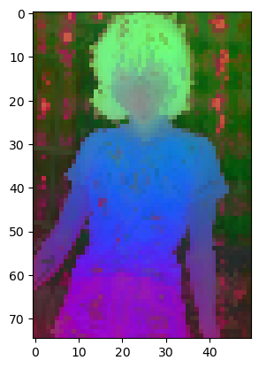
import torch
import torchvision.transforms as T
import matplotlib.pyplot as plt
import numpy as np
import matplotlib.image as mpimg
from PIL import Image
from sklearn.decomposition import PCA
import matplotlib

patch_h = 75
patch_w = 50
feat_dim = 384

transform = T.Compose([
    T.GaussianBlur(9, sigma=(0.1, 2.0)),
    T.Resize((patch_h * 14, patch_w * 14)),
    T.CenterCrop((patch_h * 14, patch_w * 14)),
    T.ToTensor(),
    T.Normalize(mean=(0.485, 0.456, 0.406), std=(0.229, 0.224, 0.225)),
])

dinov2_vits14 = torch.hub.load('', 'dinov2_vits14',source='local').cuda()

features = torch.zeros(4, patch_h * patch_w, feat_dim)
imgs_tensor = torch.zeros(4, 3, patch_h * 14, patch_w * 14).cuda()

img_path = f'/kaggle/input/demo-image/1 (4).png'
img = Image.open(img_path).convert('RGB')
imgs_tensor[0] = transform(img)[:3]
with torch.no_grad():
    features_dict = dinov2_vits14.forward_features(imgs_tensor)
    features = features_dict['x_norm_patchtokens']

features = features.reshape(4 * patch_h * patch_w, feat_dim).cpu()
pca = PCA(n_components=3)
pca.fit(features)
pca_features = pca.transform(features)
pca_features[:, 0] = (pca_features[:, 0] - pca_features[:, 0].min()) / (pca_features[:, 0].max() - pca_features[:, 0].min())

pca_features_fg = pca_features[:, 0] > 0.3
pca_features_bg = ~pca_features_fg

b = np.where(pca_features_bg)
pca.fit(features[pca_features_fg])
pca_features_rem = pca.transform(features[pca_features_fg])
for i in range(3):
    pca_features_rem[:, i] = (pca_features_rem[:, i] - pca_features_rem[:, i].min()) / (pca_features_rem[:, i].max() - pca_features_rem[:, i].min())
    # transform using mean and std, I personally found this transformation gives a better visualization
    # pca_features_rem[:, i] = (pca_features_rem[:, i] - pca_features_rem[:, i].mean()) / (pca_features_rem[:, i].std() ** 2) + 0.5
pca_features_rgb = pca_features.copy()
pca_features_rgb[pca_features_fg] = pca_features_rem
pca_features_rgb[b] = 0
pca_features_rgb = pca_features_rgb.reshape(4, patch_h, patch_w, 3)
plt.imshow(pca_features_rgb[0][...,::-1])
plt.savefig('features.png')
plt.show()
plt.close()
以下是代码的逐行中文解读:
import torch
import torchvision.transforms as T
import matplotlib.pyplot as plt
import numpy as np
import matplotlib.image as mpimg
from PIL import Image
from sklearn.decomposition import PCA
import matplotlib
# 设置补丁(patch)的高度和宽度
patch_h = 75
patch_w = 50
# 特征维度
feat_dim = 384
# 定义图像转换操作
transform = T.Compose([
    T.GaussianBlur(9, sigma=(0.1, 2.0)),  # 高斯模糊
    T.Resize((patch_h * 14, patch_w * 14)),  # 调整图像大小
    T.CenterCrop((patch_h * 14, patch_w * 14)),  # 中心裁剪
    T.ToTensor(),  # 转换为张量
    T.Normalize(mean=(0.485, 0.456, 0.406), std=(0.229, 0.224, 0.225)),  # 标准化
])
# 使用torch.hub加载dinov2_vits14模型并移***CUDA设备
dinov2_vits14 = torch.hub.load('', 'dinov2_vits14', source='local').cuda()
# 创建用于存储特征和图像张量的零张量
features = torch.zeros(4, patch_h * patch_w, feat_dim)
imgs_tensor = torch.zeros(4, 3, patch_h * 14, patch_w * 14).cuda()
# 图像路径
img_path = f'/kaggle/input/demo-image/1 (4).png'
# 打开图像并转换为RGB模式
img = Image.open(img_path).convert('RGB')
# 对图像进行转换操作,并将其存储在imgs_tensor的***个位置
imgs_tensor[0] = transform(img)[:3]
# 禁用梯度计算
with torch.no_grad():
    # 将图像张量传递给dinov2_vits14模型获取特征
    features_dict = dinov2_vits14.forward_features(imgs_tensor)
    features = features_dict['x_norm_patchtokens']

# 重塑特征形状为(4 * patch_h * patch_w, feat_dim)
features = features.reshape(4 * patch_h * patch_w, feat_dim).cpu()
# 创建PCA对象并拟合特征
pca = PCA(n_components=3)
pca.fit(features)
# 对PCA转换后的特征进行归一化处理
pca_features = pca.transform(features)
pca_features[:, 0] = (pca_features[:, 0] - pca_features[:, 0].min()) / (pca_features[:, 0].max() - pca_features[:, 0].min())
# 根据阈值进行前景和背景的区分
pca_features_fg = pca_features[:, 0] > 0.3
pca_features_bg = ~pca_features_fg
# 查找背景特征的索引
b = np.where(pca_features_bg)
# 对前景特征再次进行PCA转换
pca.fit(features[pca_features_fg])
pca_features_rem = pca.transform(features[pca_features_fg])
# 对前景特征进行归一化处理
for i in range(3):
    pca_features_rem[:, i] = (pca_features_rem[:, i] - pca_features_rem[:, i].min()) / (pca_features_rem[:, i].max() - pca_features_rem[:, i].min())
    # 使用均值和标准差进行转换,个人发现这种转换方式可以得到更好的可视化效果
    # pca_features_rem[:, i] = (pca_features_rem[:, i] - pca_features_rem[:, i].mean()) / (pca_features_rem[:, i].std() ** 2) + 0.5
# 创建RGB特征数组
pca_features_rgb = pca_features.copy()
# 替换前景特征为转换后的特征
pca_features_rgb[pca_features_fg] = pca_features_rem
# 将背景特征设置为0
pca_features_rgb[b] = 0
# 重塑特征形状为(4, patch_h, patch_w, 3)
pca_features_rgb = pca_features_rgb.reshape(4, patch_h, patch_w, 3)
# 显示***个图像的RGB特征
plt.imshow(pca_features_rgb[0][...,::-1])
plt.savefig('features.png')
plt.show()
plt.close()
这段代码的功能是对给定的图像进行一系列处理和特征提取,并使用PCA对特征进行降维。然后,根据特定阈值对前景和背景进行区分,***后将特征可视化为RGB图像。请注意,其中的具体数值和路径可能需要根据您的实际数据和环境进行调整。
print(features)
print(features.shape)
我们的输出结果为:
tensor([[-1.3500, -4.8793, -1.4393,  ...,  2.3347,  1.6834, -2.9632],
        [-0.4650, -6.4163, -1.5503,  ...,  2.2055,  2.5527, -3.2553],
        [-0.6371, -6.2615, -0.7516,  ...,  3.1827,  2.3861, -2.6838],
        ...,
        [ 1.9385,  0.0726, -0.5395,  ...,  0.3876, -1.4914, -4.5422],
        [ 1.6399, -0.0860,  0.4701,  ...,  1.0180, -0.8897, -5.2614],
        [ 1.6084, -0.0669,  0.7341,  ...,  1.0633, -0.9713, -5.3548]])
torch.Size([15000, 384])
降维后的特征为:
print(pca_features)
print(pca_features.shape)
输出的结果为:
[[  0.81004055   2.458559    12.11051576]
 [  0.79562888   5.65071716  10.84007045]
 [  0.82050109   5.55007889   9.05274001]
 ...
 [  0.27618588 -18.96898667  19.48198916]
 [  0.31861323 -12.21414371  14.19802898]
 [  0.34356016 -10.82144825  13.74648131]]
(15000, 3)
features_dict
我们看一下字典的构成:
{'x_norm_clstoken': tensor([[ 2.2549, -1.5661,  4.4978,  ...,  1.4984, -5.8642, -0.8560],
         [ 1.8816,  2.4343,  1.4931,  ..., -1.3401, -2.5460,  1.3967],
         [ 1.8816,  2.4343,  1.4931,  ..., -1.3401, -2.5460,  1.3967],
         [ 1.8816,  2.4343,  1.4931,  ..., -1.3401, -2.5460,  1.3967]],
        device='cuda:0'),
 'x_norm_patchtokens': tensor([[[-1.3500, -4.8793, -1.4393,  ...,  2.3347,  1.6834, -2.9632],
          [-0.4650, -6.4163, -1.5503,  ...,  2.2055,  2.5527, -3.2553],
          [-0.6371, -6.2615, -0.7516,  ...,  3.1827,  2.3861, -2.6838],
          ...,
          [-0.8778, -0.0251, -0.2867,  ...,  4.7801, -2.0887, -4.5910],
          [-1.2309,  0.2852,  0.7693,  ...,  5.0635, -1.1529, -6.0175],
          [-1.7551,  1.1333, -0.0898,  ...,  4.1885, -3.3197, -5.7227]],

         [[ 0.9131, -4.9736, -0.6238,  ...,  0.2835, -0.3494, -0.4916],
          [ 1.0967, -6.0392, -0.7900,  ...,  0.2323,  0.0510,  0.0176],
          [ 1.3852, -5.8056, -1.2573,  ...,  0.0549, -0.3270, -0.4510],
          ...,
          [ 1.9385,  0.0726, -0.5395,  ...,  0.3877, -1.4914, -4.5422],
          [ 1.6399, -0.0860,  0.4701,  ...,  1.0180, -0.8897, -5.2614],
          [ 1.6084, -0.0669,  0.7341,  ...,  1.0633, -0.9713, -5.3548]],

         [[ 0.9131, -4.9736, -0.6238,  ...,  0.2835, -0.3494, -0.4916],
          [ 1.0967, -6.0392, -0.7900,  ...,  0.2323,  0.0510,  0.0176],
          [ 1.3852, -5.8056, -1.2573,  ...,  0.0549, -0.3270, -0.4510],
          ...,
          [ 1.9385,  0.0726, -0.5395,  ...,  0.3877, -1.4914, -4.5422],
          [ 1.6399, -0.0860,  0.4701,  ...,  1.0180, -0.8897, -5.2614],
          [ 1.6085, -0.0669,  0.7341,  ...,  1.0633, -0.9713, -5.3548]],

         [[ 0.9131, -4.9736, -0.6238,  ...,  0.2835, -0.3494, -0.4916],
          [ 1.0967, -6.0392, -0.7900,  ...,  0.2323,  0.0510,  0.0176],
          [ 1.3852, -5.8056, -1.2573,  ...,  0.0549, -0.3270, -0.4511],
          ...,
          [ 1.9385,  0.0726, -0.5395,  ...,  0.3876, -1.4914, -4.5422],
          [ 1.6399, -0.0860,  0.4701,  ...,  1.0180, -0.8897, -5.2614],
          [ 1.6084, -0.0669,  0.7341,  ...,  1.0633, -0.9713, -5.3548]]],
        device='cuda:0'),
 'x_prenorm': tensor([[[ 4.7546e-01, -3.4794e-02,  1.1905e+00,  ...,  3.3896e-01,
           -1.2591e+00, -8.1724e-03],
          [-5.2994e-01, -3.0311e-01, -2.0162e-01,  ...,  9.4372e-01,
            8.7399e-01, -3.2527e-01],
          [-1.5728e-01, -3.9359e-01, -2.1482e-01,  ...,  9.0485e-01,
            1.2325e+00, -3.3923e-01],
          ...,
          [-4.9091e-01,  1.1081e-02,  1.9814e-01,  ...,  2.0630e+00,
           -8.5562e-01, -7.6588e-01],
          [-6.0861e-01,  5.2204e-02,  6.6299e-01,  ...,  2.1127e+00,
           -3.8590e-01, -9.7335e-01],
          [-9.3785e-01,  1.2485e-01,  3.0359e-01,  ...,  1.9137e+00,
           -1.5223e+00, -1.0352e+00]],

         [[ 4.4059e-01,  1.4807e-01,  5.9425e-01,  ..., -3.4851e-01,
           -6.1687e-01,  2.0463e-01],
          [ 3.1511e-01, -3.3073e-01,  9.0955e-02,  ...,  1.3627e-01,
            1.8562e-02,  4.2850e-02],
          [ 3.8695e-01, -4.1345e-01,  2.8734e-02,  ...,  1.1916e-01,
            1.8061e-01,  1.2469e-01],
          ...,
          [ 6.3855e-01,  1.9967e-03,  5.6187e-02,  ...,  1.0780e-01,
           -5.0606e-01, -6.6095e-01],
          [ 5.6617e-01,  4.9071e-03,  4.8375e-01,  ...,  3.7527e-01,
           -2.6194e-01, -7.9524e-01],
          [ 5.6790e-01,  1.4408e-02,  6.0538e-01,  ...,  4.0537e-01,
           -2.9182e-01, -8.1226e-01]],

         [[ 4.4059e-01,  1.4807e-01,  5.9424e-01,  ..., -3.4851e-01,
           -6.1687e-01,  2.0463e-01],
          [ 3.1511e-01, -3.3073e-01,  9.0957e-02,  ...,  1.3627e-01,
            1.8564e-02,  4.2850e-02],
          [ 3.8695e-01, -4.1345e-01,  2.8733e-02,  ...,  1.1916e-01,
            1.8061e-01,  1.2469e-01],
          ...,
          [ 6.3855e-01,  1.9971e-03,  5.6186e-02,  ...,  1.0780e-01,
           -5.0606e-01, -6.6095e-01],
          [ 5.6617e-01,  4.9067e-03,  4.8375e-01,  ...,  3.7527e-01,
           -2.6194e-01, -7.9524e-01],
          [ 5.6790e-01,  1.4408e-02,  6.0538e-01,  ...,  4.0536e-01,
           -2.9182e-01, -8.1226e-01]],

         [[ 4.4059e-01,  1.4807e-01,  5.9424e-01,  ..., -3.4851e-01,
           -6.1687e-01,  2.0463e-01],
          [ 3.1511e-01, -3.3073e-01,  9.0956e-02,  ...,  1.3627e-01,
            1.8562e-02,  4.2849e-02],
          [ 3.8695e-01, -4.1344e-01,  2.8735e-02,  ...,  1.1916e-01,
            1.8061e-01,  1.2469e-01],
          ...,
          [ 6.3855e-01,  1.9964e-03,  5.6189e-02,  ...,  1.0780e-01,
           -5.0607e-01, -6.6095e-01],
          [ 5.6617e-01,  4.9066e-03,  4.8375e-01,  ...,  3.7527e-01,
           -2.6194e-01, -7.9524e-01],
          [ 5.6790e-01,  1.4408e-02,  6.0538e-01,  ...,  4.0537e-01,
           -2.9182e-01, -8.1226e-01]]], device='cuda:0'),
 'masks': None}
我们换一种可视化的方法:
patch_h = 75
patch_w = 50
feat_dim = 384

transform = T.Compose([
    T.GaussianBlur(9, sigma=(0.1, 2.0)),
    T.Resize((patch_h * 14, patch_w * 14)),
    T.CenterCrop((patch_h * 14, patch_w * 14)),
    T.ToTensor(),
    T.Normalize(mean=(0.485, 0.456, 0.406), std=(0.229, 0.224, 0.225)),
])

dinov2_vits14 = torch.hub.load('', 'dinov2_vits14',source='local').cuda()

features = torch.zeros(4, patch_h * patch_w, feat_dim)
imgs_tensor = torch.zeros(4, 3, patch_h * 14, patch_w * 14).cuda()

img_path = f'/kaggle/input/demo-image/1 (4).png'
img = Image.open(img_path).convert('RGB')
imgs_tensor[0] = transform(img)[:3]
with torch.no_grad():
    features_dict = dinov2_vits14.forward_features(imgs_tensor)
    features = features_dict['x_norm_patchtokens']

features = features.reshape(4 * patch_h * patch_w, feat_dim).cpu()
pca = PCA(n_components=3)
pca.fit(features)
pca_features = pca.transform(features)
pca_features[:, 0] = (pca_features[:, 0] - pca_features[:, 0].min()) / (pca_features[:, 0].max() - pca_features[:, 0].min())

pca_features_fg = pca_features[:, 0] > 0.3
pca_features_bg = ~pca_features_fg

b = np.where(pca_features_bg)
pca.fit(features[pca_features_fg])
pca_features_rem = pca.transform(features[pca_features_fg])
for i in range(3):
    # transform using mean and std, I personally found this transformation gives a better visualization
    pca_features_rem[:, i] = (pca_features_rem[:, i] - pca_features_rem[:, i].mean()) / (pca_features_rem[:, i].std() ** 2) + 0.5
pca_features_rgb = pca_features.copy()
pca_features_rgb[pca_features_fg] = pca_features_rem
pca_features_rgb[b] = 0
pca_features_rgb = pca_features_rgb.reshape(4, patch_h, patch_w, 3)
plt.imshow(pca_features_rgb[0][...,::-1])
plt.savefig('features.png')
plt.show()
plt.close()
三、使用其他模型
3.1 使用vit_b14的模型
patch_h = 75
patch_w = 50
feat_dim = 768

transform = T.Compose([
    T.GaussianBlur(9, sigma=(0.1, 2.0)),
    T.Resize((patch_h * 14, patch_w * 14)),
    T.CenterCrop((patch_h * 14, patch_w * 14)),
    T.ToTensor(),
    T.Normalize(mean=(0.485, 0.456, 0.406), std=(0.229, 0.224, 0.225)),
])

dinov2_vitb14 = torch.hub.load('', 'dinov2_vitb14',source='local').cuda()

features = torch.zeros(4, patch_h * patch_w, feat_dim)
imgs_tensor = torch.zeros(4, 3, patch_h * 14, patch_w * 14).cuda()

img_path = f'/kaggle/input/demo-image/1 (4).png'
img = Image.open(img_path).convert('RGB')
imgs_tensor[0] = transform(img)[:3]
with torch.no_grad():
    features_dict = dinov2_vitb14.forward_features(imgs_tensor)
    features = features_dict['x_norm_patchtokens']

features = features.reshape(4 * patch_h * patch_w, feat_dim).cpu()
pca = PCA(n_components=3)
pca.fit(features)
pca_features = pca.transform(features)
pca_features[:, 0] = (pca_features[:, 0] - pca_features[:, 0].min()) / (pca_features[:, 0].max() - pca_features[:, 0].min())

pca_features_fg = pca_features[:, 0] > 0.3
pca_features_bg = ~pca_features_fg

b = np.where(pca_features_bg)
pca.fit(features[pca_features_fg])
pca_features_rem = pca.transform(features[pca_features_fg])
for i in range(3):
    # transform using mean and std, I personally found this transformation gives a better visualization
    pca_features_rem[:, i] = (pca_features_rem[:, i] - pca_features_rem[:, i].mean()) / (pca_features_rem[:, i].std() ** 2) + 0.5
pca_features_rgb = pca_features.copy()
pca_features_rgb[pca_features_fg] = pca_features_rem
pca_features_rgb[b] = 0
pca_features_rgb = pca_features_rgb.reshape(4, patch_h, patch_w, 3)
plt.imshow(pca_features_rgb[0][...,::-1])
plt.savefig('features.png')
plt.show()
plt.close()
3.2 使用vit_l14的模型
patch_h = 75
patch_w = 50
feat_dim = 1024

transform = T.Compose([
    T.GaussianBlur(9, sigma=(0.1, 2.0)),
    T.Resize((patch_h * 14, patch_w * 14)),
    T.CenterCrop((patch_h * 14, patch_w * 14)),
    T.ToTensor(),
    T.Normalize(mean=(0.485, 0.456, 0.406), std=(0.229, 0.224, 0.225)),
])

dinov2_vitl14 = torch.hub.load('', 'dinov2_vitl14',source='local').cuda()

features = torch.zeros(4, patch_h * patch_w, feat_dim)
imgs_tensor = torch.zeros(4, 3, patch_h * 14, patch_w * 14).cuda()

img_path = f'/kaggle/input/demo-image/1 (4).png'
img = Image.open(img_path).convert('RGB')
imgs_tensor[0] = transform(img)[:3]
with torch.no_grad():
    features_dict = dinov2_vitl14.forward_features(imgs_tensor)
    features = features_dict['x_norm_patchtokens']

features = features.reshape(4 * patch_h * patch_w, feat_dim).cpu()
pca = PCA(n_components=3)
pca.fit(features)
pca_features = pca.transform(features)
pca_features[:, 0] = (pca_features[:, 0] - pca_features[:, 0].min()) / (pca_features[:, 0].max() - pca_features[:, 0].min())

pca_features_fg = pca_features[:, 0] > 0.3
pca_features_bg = ~pca_features_fg

b = np.where(pca_features_bg)
pca.fit(features[pca_features_fg])
pca_features_rem = pca.transform(features[pca_features_fg])
for i in range(3):
    # transform using mean and std, I personally found this transformation gives a better visualization
    pca_features_rem[:, i] = (pca_features_rem[:, i] - pca_features_rem[:, i].mean()) / (pca_features_rem[:, i].std() ** 2) + 0.5
pca_features_rgb = pca_features.copy()
pca_features_rgb[pca_features_fg] = pca_features_rem
pca_features_rgb[b] = 0
pca_features_rgb = pca_features_rgb.reshape(4, patch_h, patch_w, 3)
plt.imshow(pca_features_rgb[0][...,::-1])
plt.savefig('features.png')
plt.show()
plt.close()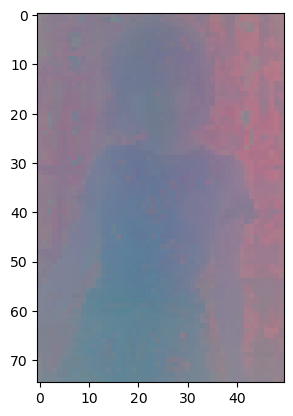
3.3 使用vit_g14的模型
patch_h = 75
patch_w = 50
feat_dim = 1536

transform = T.Compose([
    T.GaussianBlur(9, sigma=(0.1, 2.0)),
    T.Resize((patch_h * 14, patch_w * 14)),
    T.CenterCrop((patch_h * 14, patch_w * 14)),
    T.ToTensor(),
    T.Normalize(mean=(0.485, 0.456, 0.406), std=(0.229, 0.224, 0.225)),
])

dinov2_vitg14 = torch.hub.load('', 'dinov2_vitg14',source='local').cuda()

features = torch.zeros(4, patch_h * patch_w, feat_dim)
imgs_tensor = torch.zeros(4, 3, patch_h * 14, patch_w * 14).cuda()

img_path = f'/kaggle/input/demo-image/1 (4).png'
img = Image.open(img_path).convert('RGB')
imgs_tensor[0] = transform(img)[:3]
with torch.no_grad():
    features_dict = dinov2_vitg14.forward_features(imgs_tensor)
    features = features_dict['x_norm_patchtokens']

features = features.reshape(4 * patch_h * patch_w, feat_dim).cpu()
pca = PCA(n_components=3)
pca.fit(features)
pca_features = pca.transform(features)
pca_features[:, 0] = (pca_features[:, 0] - pca_features[:, 0].min()) / (pca_features[:, 0].max() - pca_features[:, 0].min())

pca_features_fg = pca_features[:, 0] > 0.3
pca_features_bg = ~pca_features_fg

b = np.where(pca_features_bg)
pca.fit(features[pca_features_fg])
pca_features_rem = pca.transform(features[pca_features_fg])
for i in range(3):
    # transform using mean and std, I personally found this transformation gives a better visualization
    pca_features_rem[:, i] = (pca_features_rem[:, i] - pca_features_rem[:, i].mean()) / (pca_features_rem[:, i].std() ** 2) + 0.5
pca_features_rgb = pca_features.copy()
pca_features_rgb[pca_features_fg] = pca_features_rem
pca_features_rgb[b] = 0
pca_features_rgb = pca_features_rgb.reshape(4, patch_h, patch_w, 3)
plt.imshow(pca_features_rgb[0][...,::-1])
plt.savefig('features.png')
plt.show()
plt.close()

发表评论:
◎欢迎参与讨论,请在这里发表您的看法、交流您的观点。